
VLOOKUP is an extremely useful function for finding information in one column and then returning information in a column to the right in the same row. Learn how to utilize Excel's VLOOKUP function to simplify your data search.
Let's Look at an Example
VLOOKUP is often used to re-organize data that exists in a Pivot Table.
=VLOOKUP (Lookup value, Table Array, Column Index number, Range Lookup)
| Lookup Value: | the cell that has the value being looked-up |
| Table Array | the cell array where the data is kept |
| Column Number | the number of the column in the array where the result will be found |
| Range Lookup | False (0) = exact match, True (1) = closest match, without going over |
*NOTE: the Look-Up Value must be in the first column of Table Array
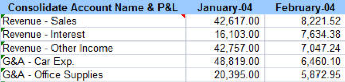
Example: We could look up” “Revenue – Sales and have it return “February 2004” value of $8,221.52
Things to remember when creating your VLOOKUP
- If you combine MATCH with VLOOKUP, the two lookup values depend on what each function is locating.
- Your lookup table array is always “chunky”- it’s a contiguous block of text, starting with the column in which your lookup value is found
- The column index can be a fixed number or a number returned by a suitable MATCH formula.
Common errors
- Adding/deleting a column within the table
- Lookup value is not identical to table value
- Duplicate lookup values return only the first one
Learn More About Excel
Discover all the hidden gems and game-changing applications in Excel through our robust Microsoft Office classes in NYC and Excel training courses. Our expert instructors will guide you every step of the way and turn you into an Excel wizard in no time. Sign up today!
For approximate matching (TRUE or an omitted fourth argument), sort the first column of the lookup table in ascending order. Use FALSE for an exact match when a nearby value would be incorrect.