
In this article, we give a quick overview of what conditional formatting is and then dive deeper into some of the practical applications of it.
What is conditional formatting?
Conditional formatting is a feature in Excel that allows us to format our cells based on a set of conditions. You are able to assign different colors or formats to cells based on your desired criteria which can be helpful in various contexts.
Why should you use conditional formatting?
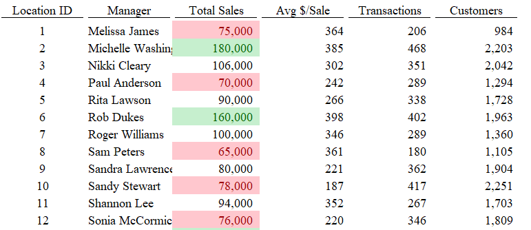
Conditional formatting is especially useful to visually get quick insights from a dataset. Say we have a dataset that has a list of our locations, with their manager, total sales, number of transactions, avg$ per sale, and total customers. At first glance, we can’t really make much of all the numbers in the sheet. Once we set up some conditional formatting we may be able to make better sense of it all. Our first exercise will be to identify managers with less than $80K in sales and to do this we will go ahead and highlight the sales column, then hit conditional formatting on the top menu, and create a Cell Rule for Less Than 80,000 to fill with dark red text. This will highlight all sales values below 80,000 with dark red text so we can easily see the underperformers. Our second exercise that builds off the first will be to find the overperformers by highlighting the list of sales and adding conditional formatting for Greater Than 120,000 and fill that with dark green text. Now we can see the underperformers in red and the overperformers in green.
Another use of conditional formatting is to identify duplicate values. In that same list of managers, we can find out if any managers are working in multiple stores to identify any staffing needs. To do this in Excel, we can highlight the list of managers and go up to conditional formatting and select Duplicate Values and highlight that in yellow.
More Advanced Applications of Conditional Formatting
Some more advanced things we can do with conditional formatting are finding the tops and bottoms of our lists, creating data bars, and making color scales for our data. Using the Tops/Bottom Rules option in conditional formatting allows us to quickly see the top/bottom 10% of our dataset, the top/bottom 10 items, or highlight the values above and/or below the average. Using the Data Bars option with conditional formatting we can create a small visual within our cells representing the scale of the value in each cell compared to another with a bar. Lastly, we can use color scales to completely color-code our data from the highest values in green and lowest values in red and everything in between on that scale or vice versa.
Learn More Useful Techniques
See our Excel classes to learn more techniques like this in hands-on training or see our other classes pages here: